
As a frequent user of excel, at what I would consider advanced-level expertise, I spend my days flying through data connections, pivots, all kinds of complex formulas, and even a dash of VBA. But there was still one hurdle I hadn’t jumped. For some odd reason those squiggly brackets { } (technically I believe they’re called “braces”) had intimidated me from dabbling in the world of arrays. Something felt unnatural about hitting ctrl + shift + enter before exiting a formula. What magic would happen behind the scenes if I pushed those buttons simultaneously? I understood the logic and language of Excel, so asking it to “work differently” just seemed bizarre. I found myself working around actually using arrays by means of extra columns, pivots, and very elaborate lookups and formulas.
This past week, however, I faced my fear and jumped in… three keys at a time!
Game changer!
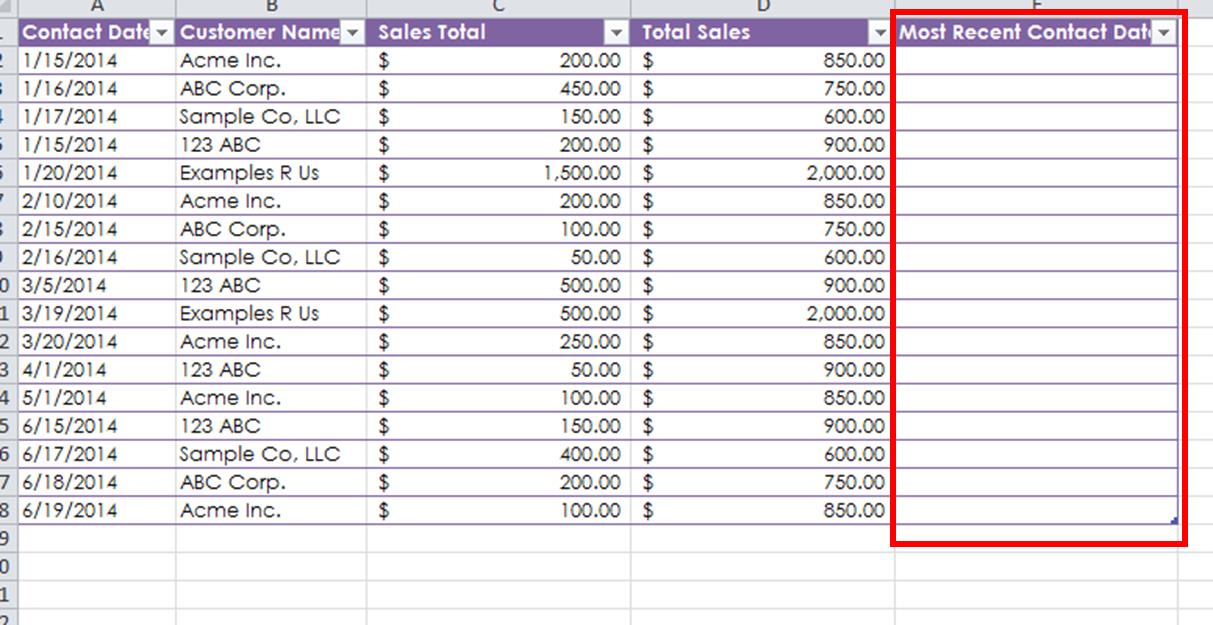
Imagine you have a list of contact dates and clients. You want to figure out how recently each person has been contacted by running a quick summary on the data. Sure, you could throw a pivot on the data, but what if you needed it in the table format? There is not a “MAXIF” formula to perform this action. In fact, for all its strengths, there is a gap on available “IF” formulas in Excel. Enter-in arrays! Arrays give you the power to combine formulas that analyze data in tabular form without having to pivot the data.
Here’s how it works:
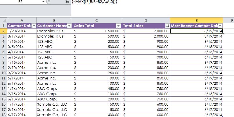
Let’s say you have a list of sales, and you want to be able to reach out to clients with whom you haven’t spoken in a while. Knowing the last contact date alongside their YTD sales will help you make sure that you are staying on top of communication with your best customers. Here’s a list of sales with contact dates. We can easily throw a “SUMIF” formula in to calculate the running total, per customer, per line. But finding out the most recent (or “max”) date is not so easy, because you cannot make a “MAXIF” formula. Instead, we can “nest” them with an array.
In everyday language, we need the formula to perform the following tasks:
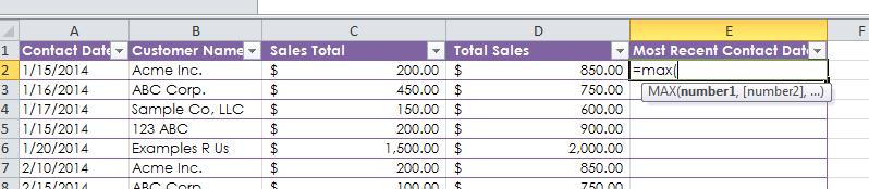
=MAX(number1, number2,…)
where the numbers are all in column A, “Contact Date.” If we just do MAX, it won’t take the customer into account. We need to add a criterion to also look for the max date of that customer.
In theory it should be this:
=MAX(IF(Customer Name = This Row’s Customer Name, THEN return the Max date from column A, OTHERWISE return a 0)
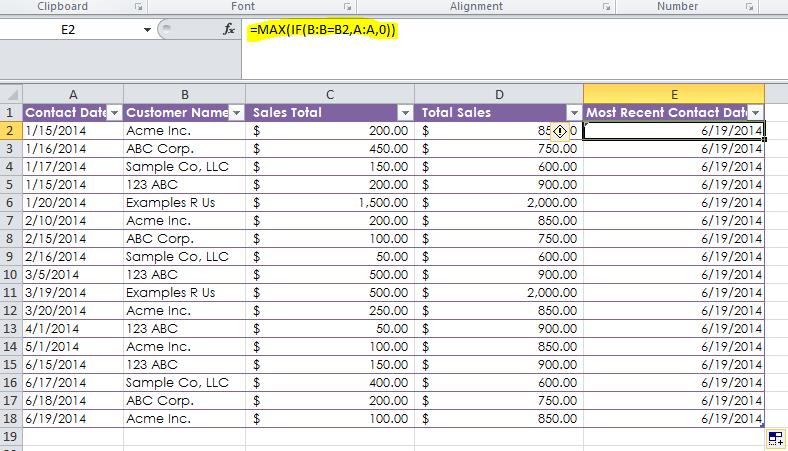
Unfortunately it doesn’t wrap the IF with the MAX and it produces a result that is the max overall. So let’s jump into those scary squiggly braces and see what we can do.
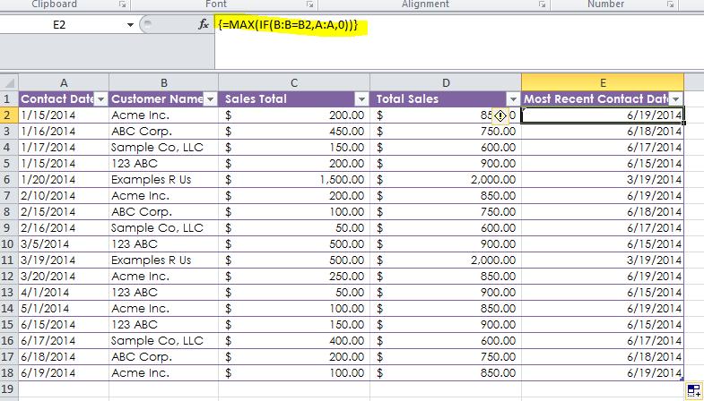
When you use the exact same formula — but before hitting enter at the end — instead, hold down CTRL + SHIFT + ENTER. You’ll see that Excel adds braces { } around the formula. When you copy this down, the formula magically evaluates both conditions across all the data you’ve selected. Voila! You have now added analytics to your table.
NOTE: You cannot simply add braces to your formulas to make this happen. You have to hit ctrl + shift + enter to make Excel perform the array formula.
So… What’s the takeaway? What can this do for you? By performing this array formula and quickly sorting my list… looks like I better reach out to Examples R Us. They’ve spent the most and it’s been the longest since they’ve been contacted.
Imagine what arrays can do to inform your business!